Variational Inference

The goal of statistical inference is to tell us things that we didn’t know based on things we do. The things want to learn about could be anything – phylogenetic trees, for example – but usually we’ll talk about numerical summaries, like “the GDP of France”, or “the reproductive rate of covid-19”. In mathematical notation we’ll label the set of numbers we don’t know $\theta \in \mathbb R^n$ (as in, $\theta$ is a list of $n$ unknown numbers) and the numbers we do know $X \in \mathbb R^m$.

However, we don’t usually expect a single right answer, like “$\theta$ is $5$”. Instead we want a range of plausible answers, like “$\theta$ is probably between $4$ and $6$”. To do this we use a function $P(\theta)$ which, given a guess for what $\theta$ could be, tells us how plausible it is – a probability distribution. When we see new data $X$, we want to update what we currently think is plausible $P(\theta)$ (aka the prior) to a new distribution $Q(\theta)$ (the posterior). $Q$ becomes our new $P$ and we can rinse and repeat as new information comes in.

Bayes’ rule makes the process of getting $Q$ from $P$ look simple:

$$ Q(\theta) = \frac{P(X,\theta)}{P(X)} $$

$$P(X, \theta)$ is very easy to get, in most cases. It’s the function we write down when we use a probabilistic programming language (PPL) to describe how $X$ and $\theta$, the knowns and unknowns – the data and the parameters – are related. But $P(X)$, the marginal likelihood of the data, turns out to be much harder. To get it from $P(X, \theta)$ we’d have to integrate over all $\theta$:

$$P(X) = \int P(X,\theta),d\theta$$

We often have thousands of $\theta$ parameters, which makes this integral impossible analytically. That means we need a workaround. One option is to use MCMC, which lets us sample from $Q(\theta)$ without knowing $P(X)$. Another is variational inference, or VI, in which we try to turn this tricky integral into an optimisation problem instead.

Neat Little Rows

To frame inference as optimisation, we can make up a candidate distribution $\hat Q(\theta)$ which has parameters we can tune, and then try to minimise the difference $D(\hat Q, Q)$ between the candidate $\hat Q$ and the true posterior $Q$. (For example, we might assume each parameter in $\theta$ is an independent Gaussian, and we can tweak each mean and variance to improve the fit.)

There are a few ways to measure how different distributions are. One particularly useful one is the KL divergence, defined as

$$ \begin{aligned} D_{KL}(\hat Q, Q) &= \int \hat Q(\theta) \log(\frac{\hat Q(\theta)}{Q(\theta)}) \,d\theta \\ &= E_{\hat Q}[ \log(\frac{\hat Q(\theta)}{Q(\theta)}) ] \end{aligned} $$

where $E_{\hat Q}[f(\theta)$] means the expected value of $f(\theta)$, given $\theta \sim \hat Q$. The divergence is always positive, and if $D_{KL} = 0$ then $\hat Q = Q$ (the two distributions are identical).

At first this looks circular; we can approxmiate $Q$ if we minimise a value that we need $Q$ to calculate. But some magic happens if we replace $Q$ with its definition per Bayes’ rule.

$$ \begin{aligned} D_{KL}(\hat Q, Q) &= E_{\hat Q}[ \log(\frac{\hat Q(\theta) P(X)}{P(X, \theta)}) ] \\ &= E_{\hat Q}[ \log(\hat Q(\theta)) - \log(P(X, \theta)) + \log(P(X)) ] \\ &= E_{\hat Q}[ \log(\hat Q(\theta)) - \log(P(X, \theta)) ] + \log(P(X)) \end{aligned} $$

The trick here is that we can separate out $\log(P(X))$, the tricky part. Because $P(X)$ is independent of $\theta$, minimising $D_{KL}$ is the same as minimising

$$ \begin{aligned} D_{KL}(\hat Q, Q) - \log(P(X)) &= E_{\hat Q}[ \log(\hat Q(\theta)) - \log(P(X, \theta)) ] \end{aligned} $$

which is easy to calculate. Another nice feature of this approach is that it gives us a lower bound on $P(X)$ (also called the “model evidence”), because $D_{KL}$ must be positive.

$$E_{\hat Q}[ \log(P(X, \theta)) - \log(\hat Q(\theta))] \le \log(P(X))$$

(Note the sign flip; we’ll maximise this quantity to minimise $D_{KL}$.)

For this reason, the left hand side is often called the “evidence lower bound” or ELBO. Getting the model evidence as part of fitting is a particularly useful feature of VI. $P(X)$ can be used to find the probability that one model is better than another, making the choice of best model a parameter like any other. So optimising the ELBO both finds the model parameters and helps us improve the model itself.

Calculating the ELBO still involves an integral, but because it’s an expectation we can approximate it by taking samples from $\hat Q$.

$$E_{\hat Q}[f(\theta)] \approx \frac{1}{N}\sum_{\theta_i \sim \hat Q}^N f(\theta_i)$$

This means that our objective function – what we minimise by gradient descent – will be noisy rather than deterministic. But that’s OK, because deep learning has given us excellent noisy optimisers, like Adam. These optimisers are so good that we can set $N = 1$ and estimate the ELBO as we improve it.¹ We just have to maximise the objective

function objective(Q̂)
  θ = rand(Q̂)
  model(θ) - logpdf(Q̂, θ)
end

where model(θ) represents the user-defined log likelihood function (implicitly using $X$).

Grounds for Divorce

It’s worth breaking down this objective a bit, and interesting to compare it to neural networks and deep learning.

$$\log(P(X, \theta)) - \log(\hat Q(\theta))$$

The first half – call it the data term – implies that we want to maximise how likely we think the data is, which seems reasonable enough. This part is often identical in neural networks. For example, the log likelihood of a Gaussian is proportional to $-||y - \hat y||^2$ (comparing data $y$ and model output $\hat y$) – so maximising likelihood is the same as minimising mean squared error. Likewise the cross entropy loss, used for discrete data, corresponds to the likelihood of a multinomial distribution. Deep learning is secretly likelihood maximisation on a statistical model – the probability distributions are just more implicit.

The second half – the model term – is more surprising. We want $\theta$ to be as unlikely as possible, with respect to $\hat Q$. Unlike deep learning, which would find a single point estimate for $\theta$, we get a distribution of plausible $\theta$ values, and this term forces the distribution to be as spread out as possible. The two terms of this objective are like attractive and repulsive forces, pulling our estimates towards the posterior mode but also repelling them from each other.² Smearing out the distribution lets us estimate the posterior mean, which is less likely to be an artifact of noise in the data than the mode – so it’s effectively a kind of regularisation.

This supports common wisdom on overfitting. Having too many parameters is bad (it decreases the model term), but can be justified if you have enough data (which puts more weight on the data term). Measures of model quality that take these factors into account, like AIC or BIC, can be derived from $P(X)$ too.

Here’s a more information-theoretical way to view the ELBO. $E_{\hat Q}[ \log(P(X, \theta))$] is the negentropy of our data with respect to the model, or in other words, the number of bits of information in the data not explained by the model. $E_{\hat Q}[\log(\hat Q(\theta))$] is the negentropy of $\hat Q$, or in other words the amount of information stored by our model. The model effectively compresses the data, and changes in the ELBO measure how many bits are saved; information that can be compressed is likely to be pattern rather than noise.

In other words: added model complexity is only worthwhile when more than offset by better explanation of the data. Occam’s razor is Bayes’ rule in disguise!

Little Fictions

That’s all well and good in theory, but we need to know how to set up $\hat Q$. The most common option is to assume each parameter in $\theta$ is distributed as an independent Gaussian (normal distribution).

$$\theta_i \sim \mathcal{N}(\mu_i,\sigma_i)$$

We can also write this as a single multivariate Gaussian

$$\boldsymbol \theta \sim \mathcal N(\boldsymbol \mu, \boldsymbol \sigma I)$$

where $\boldsymbol \sigma I$ is the $n$-dimensional covariance matrix (with only diagonal elements).³

More explicitly, the density function $\hat Q(\boldsymbol \theta)$ will be given by

$$\hat Q(\boldsymbol \theta) = p(\boldsymbol \theta | \boldsymbol \theta \sim \mathcal N(\boldsymbol \mu, \boldsymbol \sigma I))$$

where $p(x | x \sim D)$ gives the probility density of the distribution $D$. It’s easy to sample from this distribution (just sample from each normal independently), it’s easy to calculate the ELBO, and it’s easy to update each $\mu$ and $\sigma$ with gradient descent.

This works great in many cases, but remember the assumption it depends on: that all parameters are independent of each other in the posterior. It’s useful to see what happens when we break this assumption. Consider what happens with this model:⁴

$$ \begin{aligned} x &\sim \mathcal N(0, 1) \\ y &\sim \mathcal N(0, 1) \\ x + y &\sim \mathcal N(0, ¼) \end{aligned} $$

Here $x$ and $y$ are tightly correlated. Here’s what the posterior looks like, compared to what we calculate using VI.

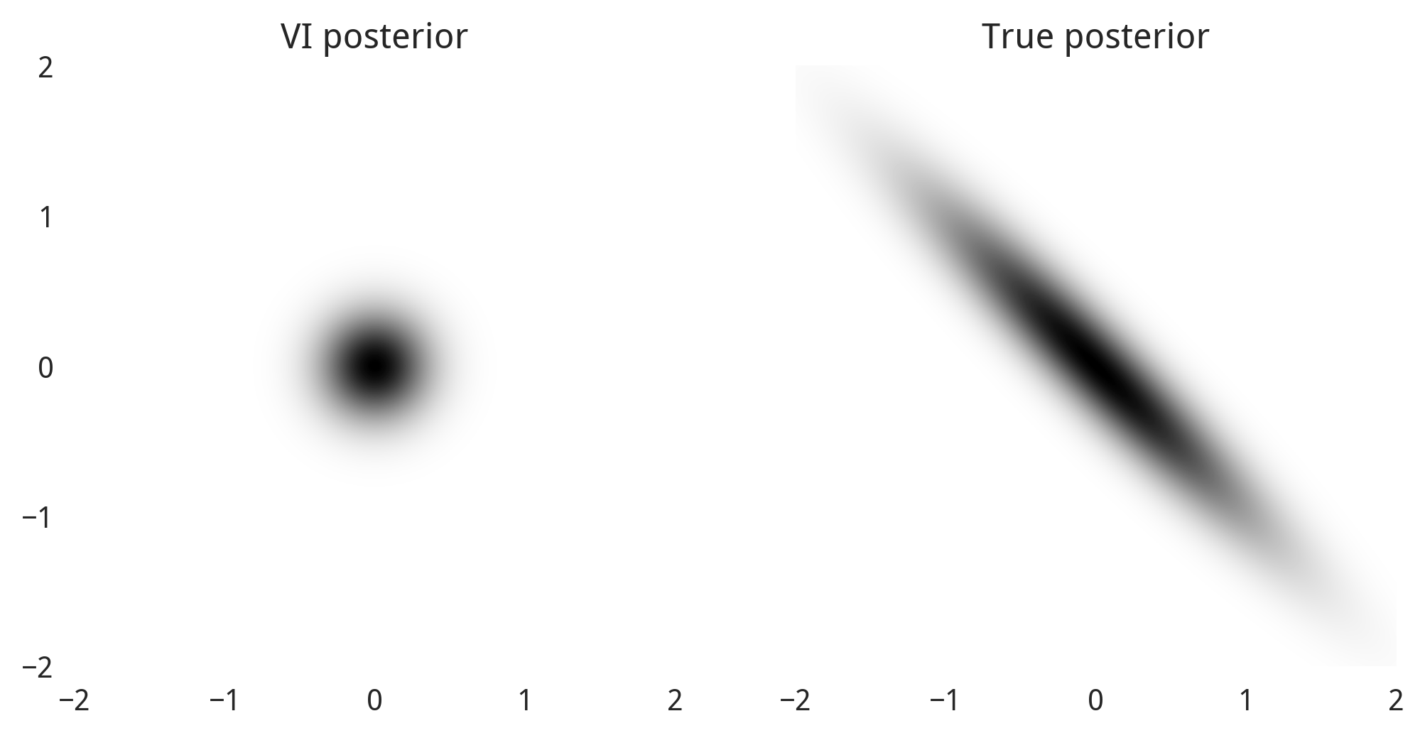
Notice that because $x$ and $y$ are treated as independent, the posterior plot can only be a horizontal or vertical elipse (or a circle). We simply can’t represent the slanted shape of the true posterior here. Instead we end up with a small disc, because being any bigger would include more unlikely values of $x$ and $y$ than likely ones.

The result is that when our parameters are correlated, we really underestimate their marginal uncertainty. This is fatal for many statistical tasks. With lots of correlated parameters the method reduces to MAP estimation, both overfitting and falsely claiming very high confidence in its results. This method can still be useful, but we’ll need to be careful how we apply it.

If our representation of the posterior distribution $\hat Q$ is too restrictive, perhaps we can loosen it up.

The Fix

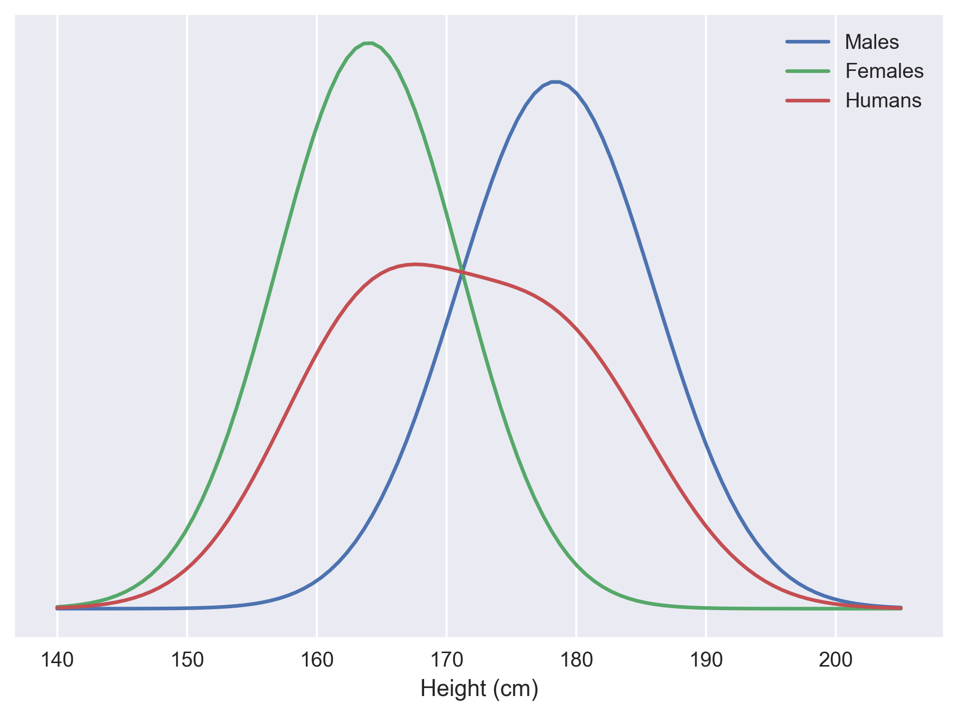
One simple way to do so is to use the idea of a mixture model, in which a more complex distribution is made up of a combination of simpler ones. Consider adult human heights: Men and women both have normally-distributed heights, but with different averages. The overall distribution is non-Gaussian but still simple to describe formally.

$$ p(\text{height}) = (p(\text{height} | \text{male}) + p(\text{height} | \text{female}))/2 $$

In our case, $\hat Q$ will be a mixture of $N$ component distributions of the kind we described above: a set of $n$ independent Gaussians. The $i$th component has a set of means $\boldsymbol \mu^i$ and deviations $\boldsymbol \sigma^i$.

$$\hat Q(\boldsymbol \theta) = \frac{1}{N}\sum_{i=1}^N p(\boldsymbol \theta | \boldsymbol \theta \sim \mathcal N(\boldsymbol \mu^i, \boldsymbol \sigma^i I))$$

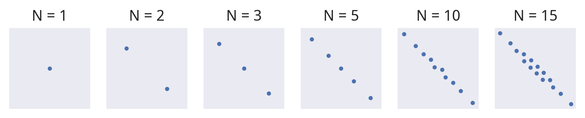
I think this idea is much easier to understand graphically. Here’s how our posterior for the $x + y$ example above looks; we can see that $N=1$ is equivalent to what we did earlier, and as $N$ increases it starts to look much more like the true posterior.

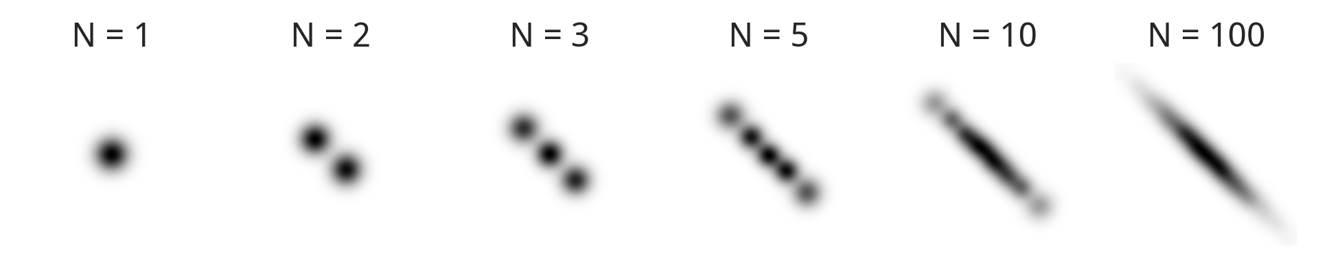
One way to look at our first approximation above is that we used a representative $n$-dimensional point, with some uncertainty over its exact location – a fuzzy disc centred at $\mu$. The mixture approach generalises this by working with $N$ representative points, a bit like a sample, each of which shows up as a fuzzy disc at $\mu_i$. Enough discs can represent a more interesting distribution, and this is reflected in the ELBO: $N=100$ has about $3\times$ better model evidence than $N=1$.

Bitten by the Tailfly

Unfortunately, extreme sparsity in the posterior still presents a challenge to most inference methods, including the one above. In these cases the result is, once again, very tight marginals around the MAP estimate, unless we use a very large number of components.

One last trick is to take the idea of a set of samples repelling each other more literally. To work backwards, imagine we already had a good set of samples via MCMC. MCMC doesn’t give us a distribution or a PDF, but with the samples we can estimate that underlying function (using a kernel density estimator, for example). Doing this will take sandpaper to the fine peaks and troughs of the true posterior, but that’s fine if we’re mainly interested in the marginal uncertainty of individual parameters.

So instead of starting with a guess for the posterior distribution $\hat Q$, start with a guess for a set of samples from the posterior; find the distribution implied by those samples; use both to approximate the ELBO; then improve the ELBO by tweaking the samples. The net result should be a representative⁵ set of points that are good enough for getting marginals.

We’ll need a way to calculate the probability density. The word “density” is not coincidental; it’s the expected number of particles in a unit volume. Given two particles in $n$-dimensional space, at a Euclidean distance of $d$ from each other, we can carve around each point a hypersphere⁶ (with volume proportional to $d^n$) and the density is $1/d^n$. We can average the density over all pairs of points to get the density at a point $\theta_i$:

$$\rho(\theta_i) = \frac{1}{N} \sum_{j \ne i}^N \frac{1}{||\theta_i-\theta_j||^n}$$

And so the ELBO, estimated using the samples that we have, is:

$$\frac{1}{N} \sum_i^N \log(P(X,\theta_i)) - \log(\rho(\theta_i))$$

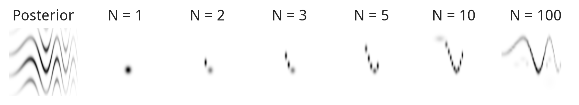
In this modeller’s testing so far, this seems to work quite well. Here’s what the resulting samples look like on our motivating example; notice that at $N=1$ it handily reduces to MAP again.

We start getting reasonable marginals at low $N$, and even on tricky high-dimensional examples (eg this time series model), we seem to either get the right marginals or overestimate them by a small factor – far better than underestimating them. The objective is also deterministic, which greatly improves fitting times. When all else fails, variational inference is a very useful trick to have up your sleeve.